Introduction to Policy Gradient

Problem Setup

For simplicity, let us first consider a one-step decision-making process (also known as a contextual bandit).

We define the following notions:

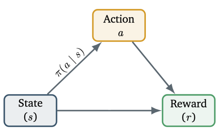
• Let $s\in \mathcal{S}$ be the state vector of the environment, describing the current situation or configuration the agent observes (for example, the position of a robot, or the market condition in trading).
• Let $a\in \mathcal{A}$ be the action taken by the agent — a decision or move that affects the environment (e.g., moving left/right, buying/selling).
• Let $r(a,s)$ denote the reward function, which assigns a numerical score to each action–state pair, indicating how desirable the action is when taken in that state.

The agent’s behavior is characterized by a policy, represented as a conditional probability distribution $\pi (a\mid s),$ which specifies the probability of selecting each possible action $a$ given the current state $s$.

The objective is to learn an optimal policy ${\pi }^{\ast }$ that maximizes the expected reward under the environment’s state distribution. Formally, we define the performance of a policy $\pi$ as

$$R({\pi }_{\theta })={\mathbb{E}}_{s\sim p_0}{\mathbb{E}}_{a\sim {\pi }_{\theta }(\cdot \mid s)}[r(a,s)],$$

which can equivalently be written as a joint expectation:

$$R(\pi )=\sum _{s,a}{p}_{\pi }(s,a)r(a,s),$$

where $p_0(s)$ denotes the (unknown) distribution of states in the environment, and

$$p_{\pi }(s,a)=p_0(s)\pi (a\mid s)$$

is the joint distribution of states and actions induced by the policy $\pi$.

In practice, the state distribution $p_0$ is rarely known in closed form; instead, we have access to a finite set of samples $\{s^{(i)}{\}}_{i=1}^N$ drawn from $p_0$, typically obtained from interaction with the environment or an existing dataset.

So far, we have

$$\begin{array}{rl}R({\pi }_{\theta })=& {\mathbb{E}}_{s\sim p_0}{\mathbb{E}}_{a\sim {\pi }_{\theta }(\cdot \mid s)}[r(a,s)]\\ =& \sum _{s,a}{p}_0(s){\pi }_{\theta }(a|s)r(a,s)\end{array}$$

Policy Gradient

In practice, the policy ${\pi }_{\theta }(a\mid s)$ is parameterized by a differentiable function. The gradient of the expected reward is:

$$\begin{array}{rl}{\nabla }_{\theta }R({\pi }_{\theta })=& {\nabla }_{\theta }(\sum _{s,a}{p}_0(s){\pi }_{\theta }(a|s)r(a,s))\\ =& \sum _{s,a}{p}_0(s){\nabla }_{\theta }{\pi }_{\theta }(a|s)r(a,s)\\ =& \sum _{s,a}{p}_0(s){\pi }_{\theta }(a|s)\frac{{\nabla }_{\theta }{\pi }_{\theta }(a|s)}{{\pi }_{\theta }(a|s)}r(a,s)\\ =& \sum _{s,a}{p}_0(s){\pi }_{\theta }(a|s){\nabla }_{\theta }\log {\pi }_{\theta }(a\mid s)r(a,s)\\ =& {\mathbb{E}}_{p_{{\pi }_{\theta }}}\left[r(a,s){\nabla }_{\theta }\log {\pi }_{\theta }(a\mid s)\right].\end{array}$$

(Used the log-derivative trick: ${\nabla }_{\theta }{\pi }_{\theta }/{\pi }_{\theta }={\nabla }_{\theta }\log {\pi }_{\theta }$.)

---

Reward Baseline

For any policy ${\pi }_{\theta }$, we can derive the following identity:

$$\begin{array}{rl}& {\mathbb{E}}_{a\sim {\pi }_{\theta }(\cdot |s)}[{\nabla }_{\theta }\log {\pi }_{\theta }(a\mid s)]\\ =& \sum _a{\pi }_{\theta }(a\mid s){\nabla }_{\theta }\log {\pi }_{\theta }(a\mid s)\\ =& \sum _a{\nabla }_{\theta }{\pi }_{\theta }(a\mid s)\\ =& {\nabla }_{\theta }\sum _a{\pi }_{\theta }(a\mid s)\\ =& {\nabla }_{\theta }1\\ =& 0.\end{array}$$

Then, we have

$$\begin{array}{rl}& {\mathbb{E}}_{p_{{\pi }_{\theta }}}[v(s){\nabla }_{\theta }\log {\pi }_{\theta }(a\mid s)]\\ =& {\mathbb{E}}_{s\sim p_0}{\mathbb{E}}_{a\sim {\pi }_{\theta }(\cdot |s)}[v(s){\nabla }_{\theta }\log {\pi }_{\theta }(a\mid s)]\\ =& {\mathbb{E}}_{s\sim p_0}(v(s){\mathbb{E}}_{a\sim {\pi }_{\theta }(\cdot |s)}[{\nabla }_{\theta }\log {\pi }_{\theta }(a\mid s)])\\ =& {\mathbb{E}}_{s\sim p_0}(v(s)\cdot 0)\\ =& 0.\end{array}$$

Hence, by the linearity of expectation, we can subtract any function $v(s)$ independent of $a$ from the reward without changing the policy gradient:

$${\nabla }_{\theta }R({\pi }_{\theta })={\mathbb{E}}_{p_{{\pi }_{\theta }}}\left[(r(a,s)-v(s)){\nabla }_{\theta }\log {\pi }_{\theta }(a\mid s)\right],$$

where $v(s)$ is any function independent of $a$.

Choosing $v(s)={\mathbb{E}}_a[r(a,s)]$ gives the advantage function:

$$A(a,s)=r(a,s)-v(s).$$

A positive $A(a,s)$ means the action performs above average.

So far, we have the policy gradient expressed as

$${\nabla }_{\theta }R({\pi }_{\theta })={\mathbb{E}}_{p_{{\pi }_{\theta }}}\left[A(a,s){\nabla }_{\theta }\log {\pi }_{\theta }(a\mid s)\right].$$

---

On-Policy Estimation

Given data $\{(s_i,a_i)\}$ with $s_i\sim p_0$ and $a_i\sim {\pi }_{\theta }(\cdot |s_i)$,

$${\nabla }_{\theta }R({\pi }_{\theta })\approx \frac{1}{n}\sum _{i=1}^n{A}_i{\nabla }_{\theta }\log {\pi }_{\theta }(a_i\mid s_i),$$

with $A_i=A(a_i,s_i)$.

Gradient ascent update (REINFORCE):

$$\theta \leftarrow \theta +ϵ{\nabla }_{\theta }R({\pi }_{\theta }).$$

Intuitively:

• $A_i>0$: increase ${\pi }_{\theta }(a_i|s_i)$;
• $A_i<0$: decrease it.

---

Connection to Weighted MLE

If data $(a_i,s_i)$ are fixed, the policy gradient equals the gradient of the $A_i$-weighted log-likelihood.

Let’s consider the following log-likelihood function:

$$\ell ({\pi }_{\theta })=\frac{1}{n}\sum _{i=1}^n{A}_i\log {\pi }_{\theta }(a_i\mid s_i).$$

Thus, policy optimization ≈ adaptive MLE with dynamic weights $A_i$.

---

Off-Policy Estimation (Importance Sampling)

If data are drawn from a behavior policy ${\pi }_{\mathrm{data}}$, using importance sampling, we have:

$$\begin{array}{rl}{\nabla }_{\theta }R({\pi }_{\theta })=& {\mathbb{E}}_{p_{{\pi }_{\mathrm{data}}}}\left[\frac{{\pi }_{\theta }(a|s)}{{\pi }_{\mathrm{data}}(a|s)}A(a,s){\nabla }_{\theta }\log {\pi }_{\theta }(a\mid s)\right]\\ \approx & \frac{1}{z}\sum _{i=1}^n{w}_i{A}_i{\nabla }_{\theta }\log {\pi }_{\theta }(a_i|s_i),\end{array}$$

where

$$w_i=\frac{{\pi }_{\theta }(a_i|s_i)}{{\pi }_{\mathrm{data}}(a_i|s_i)},$$

and the normalization factor $z$ is often taken as $z={\sum }_i{w}_i$.

---

Proximal Policy Optimization (PPO)

Proximal Point Method

Starting from ${\theta }^0$, iterate:

$${\theta }^{k+1}=\arg \underset{\theta }{\max }\{R(\theta )-\beta D(\theta ,{\theta }^k)\},$$

where $D$ measures the deviation between parameters (e.g., squared distance or KL divergence).

This forms the basis for proximal methods.

---

Proximal Gradient Descent

Approximate $R(\theta )$ by its first-order Taylor expansion:

$$R(\theta )\approx R({\theta }^k)+\nabla R({\theta }^k{)}^{\top }(\theta -{\theta }^k).$$

Then, since ${\theta }^k$ is independent of the optimization variable $\theta$, the update becomes:

$${\theta }^{k+1}=\arg \underset{\theta }{\max }\{\nabla R({\theta }^k{)}^{\top }(\theta -{\theta }^k)-\beta D(\theta ,{\theta }^k)\}.$$

Preconditioning Gradient Descent

Consider a quadratic proximal penalty:

$$D(\theta ,{\theta }^k)=\frac{1}{2}(\theta -{\theta }^k{)}^{\top }J({\theta }^k)(\theta -{\theta }^k),$$

where $J({\theta }^k)$ is a positive definite matrix, chosen by user.

Then the update has a closed-form solution:

$${\theta }^{k+1}={\theta }^k+J({\theta }^k{)}^{-1}\nabla R({\theta }^k).$$

This is known as preconditioned gradient descent.

---

Remark. Assume we use gradient descent to solve the inner loops of proximal methods. The difference from vanilla gradient descent then lies in how the reference point is updated. To see this, let us consider the following generic update rule

$${\theta }^{k+1}=\arg \underset{\theta }{\max }\{\nabla R({\theta }^k{)}^{\top }(\theta -{\theta }^k)-\beta D(\theta ,{\theta }^{ref,k})\}.$$

The proximal point framework interpolates between fast-updating methods (gradient descent) and slower, more implicit schemes, depending on how the reference point ${\theta }^{\text{ref},k}$ evolves.

• ${\theta }^{\text{ref},k}={\theta }^k$: proximal gradient descent
• ${\theta }^{\text{ref},k}={\theta }^{m\lfloor k/m\rfloor }$: inner-loop updates
• EMA of past iterates → smoother, more stable updates

---

Proximal Policy Optimization (PPO)

Applying the proximal framework to policy optimization with importance sampling:

$${\theta }^{k+1}=\arg \underset{\theta }{\max }\left\{{\mathbb{E}}_{\mathcal{D}}\right[\frac{{\pi }^{\theta }(a|s)}{{\pi }_{\mathrm{data}}(a|s)}r(a,s)]-\beta D({\pi }^{\theta }\Vert {\pi }^{{\theta }^k})\}.$$

Derivation:

We have the original formula

$${\theta }^{k+1}=\arg \underset{\theta }{\max }\{R(\theta )-\beta D(\theta ,{\theta }^k)\}$$

From off-policy estimation, we have

$$\begin{array}{rl}{\nabla }_{\theta }R({\pi }_{\theta })=& {\mathbb{E}}_{p_{{\pi }_{\mathrm{data}}}}\left[\frac{{\pi }_{\theta }(a|s)}{{\pi }_{\mathrm{data}}(a|s)}A(a,s){\nabla }_{\theta }\log {\pi }_{\theta }(a\mid s)\right]\\ =& {\mathbb{E}}_{p_{{\pi }_{\mathrm{data}}}}\left[\frac{1}{{\pi }_{\mathrm{data}}(a|s)}A(a,s){\nabla }_{\theta }{\pi }_{\theta }(a\mid s)\right]\\ =& {\mathbb{E}}_{p_{{\pi }_{\mathrm{data}}}}\left[\frac{{\nabla }_{\theta }{\pi }_{\theta }(a\mid s)}{{\pi }_{\mathrm{data}}(a|s)}A(a,s)\right]\\ =& {\nabla }_{\theta }{\mathbb{E}}_{p_{{\pi }_{\mathrm{data}}}}\left[\frac{{\pi }_{\theta }(a\mid s)}{{\pi }_{\mathrm{data}}(a|s)}A(a,s)\right]\end{array}$$

Taking integration, we have

$$\begin{array}{rl}R({\pi }_{\theta })=& {\mathbb{E}}_{p_{{\pi }_{\mathrm{data}}}}\left[\frac{{\pi }_{\theta }(a\mid s)}{{\pi }_{\mathrm{data}}(a|s)}A(a,s)\right]\end{array}$$

Substitute above to the original formula, we get the final result.

The penalty term is usually the KL divergence:

$$D({\pi }^{\theta }\Vert {\pi }^{{\theta }^k})={\mathbb{E}}_{s\sim p_0}[\mathrm{KL}({\pi }^{\theta }(\cdot |s)\Vert {\pi }^{{\theta }^k}(\cdot |s))].$$

---

Clipping Objective

PPO further introduces a clipping function:

$${\theta }^{k+1}=\arg \underset{\theta }{\max }{\mathbb{E}}_{\mathcal{D}}\left[\mathcal{C}(w_{\theta }(a,s),r(a,s))\right]-\beta D({\pi }^{\theta }\Vert {\pi }^{{\theta }^k}),$$

where $w_{\theta }(a,s)=\frac{{\pi }^{\theta }(a|s)}{{\pi }_{\mathrm{data}}(a|s)}$ and $\mathcal{C}(w,r)=\min (wr,\text{clip}(w,[1-ϵ,1+ϵ]),r)$

Different choices of penalty $D$ and clipping function yield different stability–efficiency tradeoffs.

GRPO

GRPO Basic

In GRPO case, we change the advantage function into group-relative advantage.

For a given state $s$, the policy takes $n$ different action $a_1,a_2,\cdots a_n$ .

We define the following notations:

• Let $r_i:=r(s,a_i)$, which denotes the reward for action $a_i$.
• Let $\{r_i\}$ denote the group-reward for state $s$.
• Let $\mathrm{mean}(\{r_i\})$ and $\mathrm{std}(\{r_i\})$ denote the mean and standard deviation of the gorup-reward $\{r_i\}$.

We define the advantage function for action $a_i$ as follows:

$$A_i=\frac{r_i-\mathrm{mean}(\{r_i\})}{\mathrm{std}(\{r_i\})}$$

GRPO in LLMs

In LLMs setting, we define the following notation

• The user query $Q$.
• The model response $Y=\{y_1,\cdots y_m\}$
• Response probability ${\Pi }_{i=1}^m{\pi }_{\theta }(y_i|y_{j<i},Q)$
• Response reward $R(Q,Y)$